Using PennCNV within BeadStudio/GenomeStudio via UniversalCNVAdapter

              
This note describes the procedure to run PennCNV within Illumina BeadStudio/GenomeStudio software to facilitate automatic processing and visualization of CNV calls. This procedure has been only tested on 32-bit Windows XP with ActivePerl 5.8 and BeadStudio 3.1 installation, or with ActivePerl 5.10 and GenomeStudio 2009 installation. Note: 64-bit Windows system should be compatible to most 32-bit executables, as long as all components of the program are compiled in 32-bit code; therefore, if you install 32-bit Perl in the 64-bit Windows computer, in principle PennCNV can still run without re-compilation, and this has been confirmed by some users.

Before using PennCNV within BeadStudio, the user should be aware of the some of the advantages and disadvantages. The advantage is obvious: one can simply click mouse buttons and perform CNV detection and visualization. The disadvantages are: (1) it is very slow: The CNV calling is implemented by exporting signal files from BeadStudio one by one, and then calling PennCNV again and again for each file, and each time reloading all necessary model files into memory, which is a very inefficient way to perform CNV analysis by PennCNV. (2) it does not allow flexible post-processing of CNV calling results. (3) It does not allow family-based PennCNV calls by PennCNV. In general, due to the inefficiency of running PennCNV within BeadStudio/GenomeStudio, if you have many hundred or thousand samples and you only use Windows system and you do not want to wait multiple days to run CNV analysis, you are probably better off using command line in Windows shell or in Cygwin to run PennCNV, while using the BeadStudio plug-in for validating important CNV calls in chosen samples. We have now provided auxiliary programs (visualize_cnv.pl) to transform PennCNV output directly to BeadStudio/GenomeStudio bookmarks, so that you can run PennCNV in command line, then directly import the calls to Illumina Genome Viewer for visualization.

The procedure for using PennCNV with BeadStudio/GenomeStudio is described below in step-by-step fashion.

Make sure your computer has at least 2GB (preferably 4GB) memory. (if the computer has less memory, PennCNV can still run on virtual memory, but the speed is extremely slow!) Now download PennCNV at http://www.openbioinformatics.org/penncnv/download/penncnv.latest.zip, unzip the file and then move the resulting penncnv folder into C:\penncnv\. Download the free ActivePerl for windows version 5.8 or 5.10, install the ActivePerl program with all default options (the default installation location is C:\perl, and the executable will be C:\perl\bin\perl.exe).

To make sure that PennCNV work correctly in your operating system, open a command terminal (Click “Start” button in the taskbar in the lower left of your computer screen, select “Run …”, then type “cmd.exe”), then type in “perl C:\penncnv\detect_cnv.pl” to see whether the program can run successfully (a list of command line options will be printed out in the screen).

If you have not done so, download the Illumina Universal CNV Adapter plugin from http://www.illumina.com/pagesnrn.ilmn?ID=229, and use v1 for BeadStudio and v2 for GenomeStudio. Install the program with all default options (the default installation locations is C:\Program Files\Illumina\BeadStudio 2.0\CNVAlgorithm\UniversalCNVAdapter for BeadStudio or C:\Program Files\Illumina\GenomeStudio\CNVAlgorithm\UniversalCNVAdapter\ for GenomeStudio).

Now go to the installation directory, rename the UniversalCNVAdapterPlugin.dll.config file to UniversalCNVAdapterPlugin.dll.config.bak, so that we can restore to the original settings if wanted. Next copy UniversalCNVAdapterPlugin.dll.config file from C:\penncnv\extra\ to here. This configuration file contains necessary command line options for running PennCNV through BeadStudio/GenomeStudio.

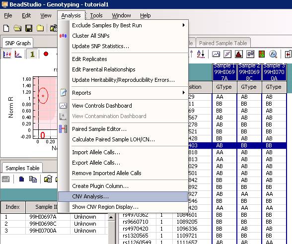
Now we can open a project file. As an example, we can use the same project file as used in the PennCNV tutorial (download here), which contains genotyping data for 3 individuals (father, mother and autistic child) within a family. (If using GenomeStudio, there will be a warning message that the file cannot be opened in BeadStudio after being opened in GenomeStudio, just click "yes" to accept this.) Click “Analysis” menu, then click “CNV analysis” (see below).

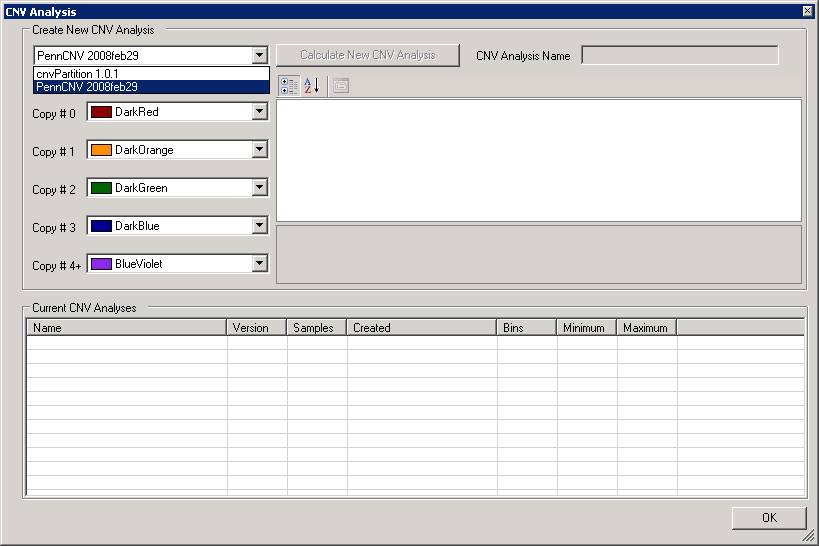
The CNV analysis dialogue will show up, now select “PennCNV” from the dropdown menu. See below:

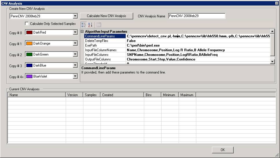
We can now change some parameters if necessary. For example, by clicking the “CommandLineParams” text box, we can change the path to the detect_cnv.pl program, or change the HMM and PFB file. Note that all the parameters are separated by comma (NOT by space!).

Additionally, note that there is a check box "Calculate only selected samples" in the window. If the user has selected one or a few samples in the "Sample Table" in BeadStudio/GenomeStudio, then checking this box will restrict the analysis to only selected samples. This option is useful to examine CNVs in specific samples if the project file contains many hundred samples.

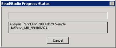
Now we can click “Calculate New CNV Analysis”, a progress dialogue will show up:

It takes about 3-5 minutes to process one sample in a modern computer. If it takes >10 minutes for one sample, then clearly something is wrong: check the computer CPU/memory usage by opening Windows Task Manager to see whether this is due to insufficient memory. The CNV call results will be given in the CNV Region Display (see below). Each colored bar represent one CNV call, while the color indicates the copy number (see legend in the upper right of the figure). If you like the generated figure, you can right click the legend area by mouse, then select “save as image…” to save a TIFF file for the CNV calls.

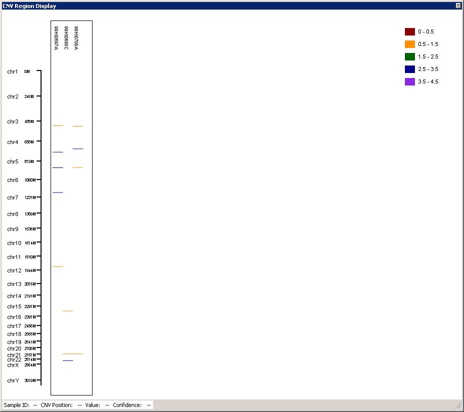
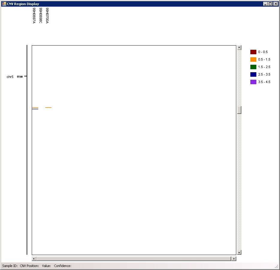
You can use the “scroll” button in mouse (middle button) to zoom in and out of particular genomic regions, when the cursor is located on top of a region of interest in the graph. For example, we can zoom in the CNV in chr5, and we can see that there are two CNVs (one deletion, one duplication) adjacent to each other in the father, and the deletion is inherited to offspring.

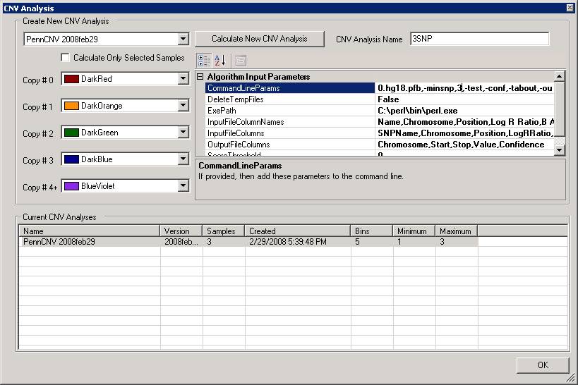
In the above calculation, we used the 10-SNP threshold for CNV calling (this means that only CNV calls containing >=10 SNPs are printed in output). Now we can try to do it again using 3-SNP threshold. We can type in a new name (for example, 3SNP) for the analysis in the “CNV Analysis Name” box, then click the textbox next to “CommandLineParams”, and change the “-minsnp,10” to “-minsnp,3” (see below).

Run the program again, we will have the following output in the “CNV region display”:

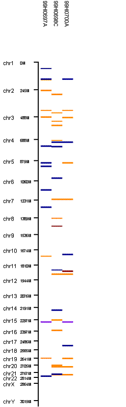
When 3-SNP threshold is used, much more CNV calls are generated.

Note that by default, PennCNV only process autosomes. To handle chrX, one need to add “,-chrx” to the command line parameters and run PennCNV again from there.

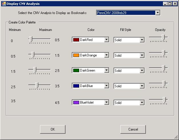
The generated CNV calls can be further visualized along the chromosome in the Illumina Genome Viewer. Click the “Tools” menu, then click “Show Genome Viewer …” to open the Genome Viewer.If using GenomeStudio, there may be a dialogue asking to select LRR and BAF for specific samples first. Next, click “View” menu, and select “CNV analysis as bookmarks” (see below). In the dropdown box, we can select the PennCNV analysis that we have just performed. It is probably a good idea to increase the default Opacity level to about 80% for easier visual identification of small CNVs in the Genome Viewer.

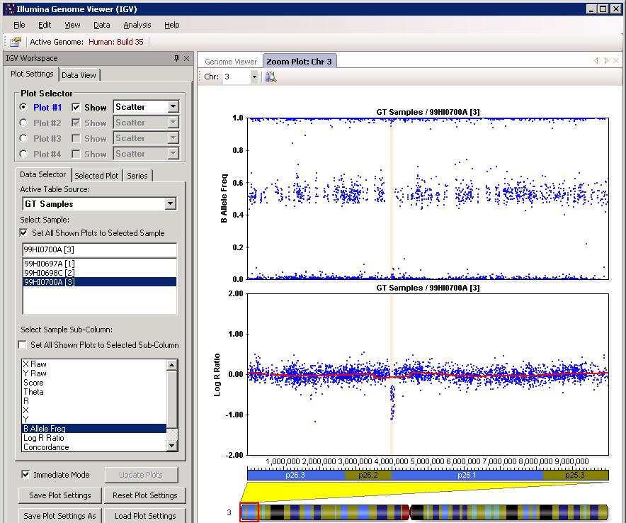
After clicking “OK”, we can then check the CNV calls visually to eliminate spurious calls. One example in BeadStudio is shown below. (However, the figure below used Human genome build 35, resulting in small discordances.). Make sure that “Immediate Mode” checkbox is selected, or one must click “Update Plots” after selecting different samples for the plot to update.

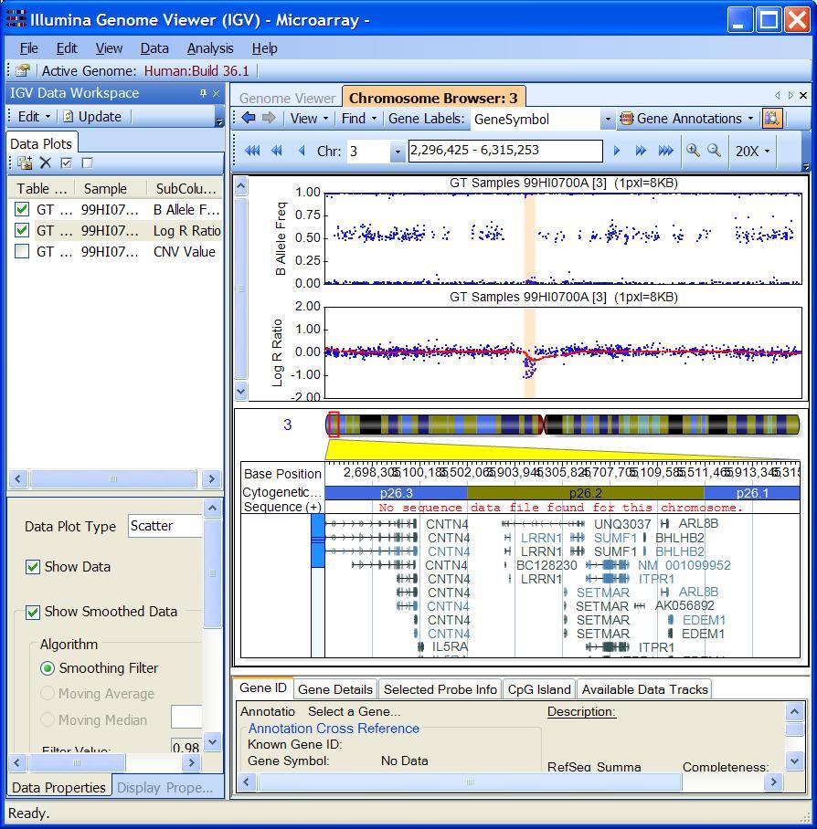
The example is shown in GenomeStudio below:

Through visual examination of the signal intensity patterns within predicted CNV region, we may be able to gain additional confidence in CNV calls, or eliminate false positive calls due to random signal fluctuation.

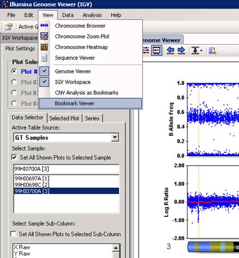
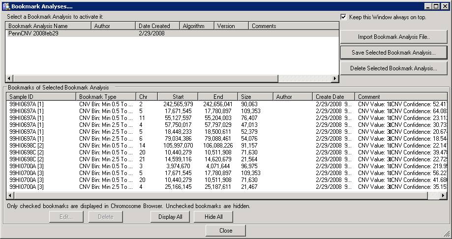
With the “Bookmark Viewer” (see below), we can examine the details of the CNV calls and export them as text files for further processing.
                      

The CNV calls can be saved as a XML file for further processing, by clicking the “Save Selected Bookmark Analysis” button. However, when you have a lot of samples, it is much easier and more informative to run PennCNV directly with command line and save the output files.