PennCNV Input File Formats

PennCNV input files are all in text formats. It requires a signal intensity file, a HMM file, a PFB file, and optionally a GCModel file. The users will need to prepare the signal intensity files in the correct formats, while all other files are bundled in the PennCNV package already. Below we describe the various input file formats, and describe the procedure to prepare the signal intensity files from various sources.
                                                        
                                                        
1 PennCNV input signal intensity files
1.1       Preparing input signal intensity files from Illumina Report
1.2       Preparing input signal intensity files from BeadStudio project files
1.3       Preparing signal intensity files from Affymetrix CEL files
1.4       Preparing signal intensity files from other types of arrays (Agilent, Nimblegen, Affy, etc)
1.4.1         Normalized signal file
1.4.2         Genotype call file
1.4.3         Genotype confidence file
1.4.4         Generating cluster file and LRR/BAF file
2 PFB (Population frequency of B allele) file
3 HMM file
4 GCModel file
5 List file

PennCNV input signal intensity files

The input signal intensity file is a text file that contains information for one marker per line, and all fields in each line are tab-delimited. One example is given below:

The first line of the file specifies the meaning for each tab-delimited column. For example, there are six fields in each line in the file, corresponding to SNP name, chromosome, position, genotype, Log R Ratio (LRR) and B Allele Frequency (BAF), respectively.

The CNV calling only requires the SNP Name, LRR and BAF values (the chromosome coordinates are annotated in the PFB file, see below). Therefore, the following input signal intensity file will work as well. Note that the relative position of LRR and BAF is different from the previous file; again the header line tells the program that the second column represents BAF values, yet the third column is LRR values.

Preparing input signal intensity files from Illumina Report

Sometimes, the user may get a text file from the genotyping center, which should contain the signal intensity values (Log R Ratio and B Allele Frequency) for all markers in all samples in a given project. The first a few lines should look like the following:

If after the [Data] line, we do not see the “SNP Name”, “Sample ID”, “B Allele Freq” and “Log R Ratio”, then it is necessary to contact the data provider and ask them to re-generate a report file that contains all these required fields. Having extra fields in the file, like the X, Y, X Raw and Y Raw fields, are just fine, but only the LRR and BAF values are useful for CNV calling.

The PennCNV package provides a convenient script to convert this long and bulk report file into individual signal intensity files for use with PennCNV calling, and each file contains information for one sample.

The output file name corresponds to the “Sample ID” field in the original report file. In the above command, the -prefix argument is used to specify the prefix of the file name (in this case, save the file to the rawdata1/ directory). We can use “-suffix .txt” to add a suffix to file name. Furthermore, we can use -numeric argument so that the output file name is in split1, split2, split3 format. In some cases, the genotyping center may provide the report file in comma-delimited format rather than tab-delimited format; the -comma argument can be used in this case to handle such files.

Preparing input signal intensity files from BeadStudio project files

In some cases, we may get the genotyping data in BeadStudio project file format (or sometimes many files in idat format, which can be built into a single project file). The goal of this section is to illustrate how to export the signal intensity data (pre-computed Log R Ratio and B Allele Freq data) from a genotyping project to a text file, so that it can be analyzed subsequently by PennCNV. We need to use a computer system with the Illumina BeadStudio software, which can be obtained probably from your microarray core facility.

For this tutorial, we can download the tutorial project file as a single tutorial_beadstudio.zip file with about 100MB (see the Download page). This project file contains genotyping data for 3 individuals (a trio), genotyped by the Illumina HumanHap550 SNP genotyping chip. (We assume that the genotype data has been clustered appropriately and that the signal intensity values have already been computed by the BeadStudio software; if not, load the appropriate *.EGT file for clusteing file, before doing any data export).
                                 
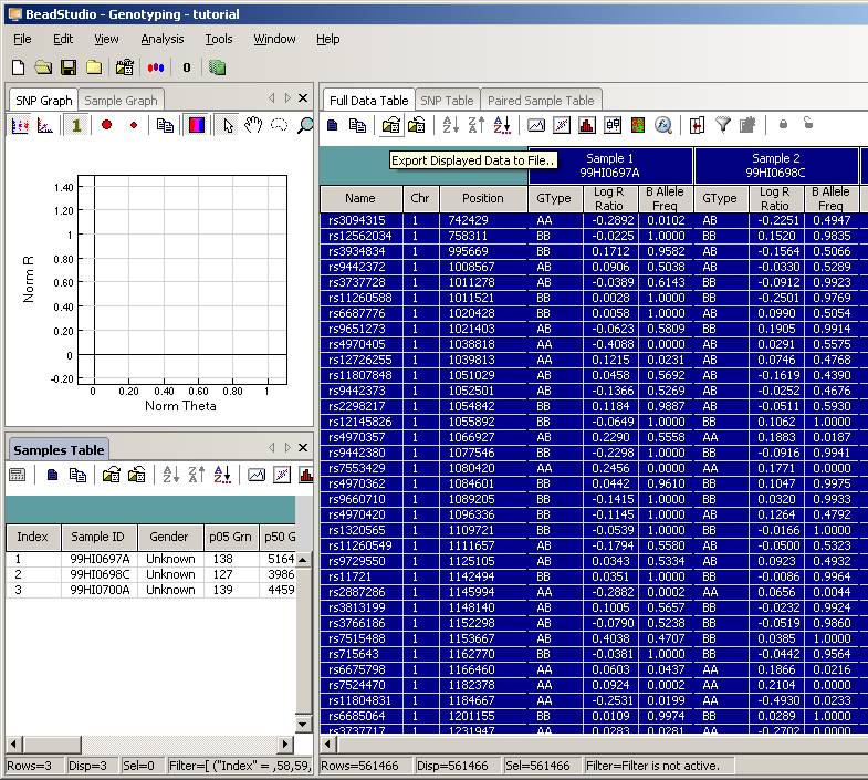
Now uncompress the ZIP file, and we will see a directory called "tutorial". Enter this directory, and then double click the project file tutorial.bsc. The BeadStudio software should be automatically invoked and the genotyping data will be loaded into the software interface:

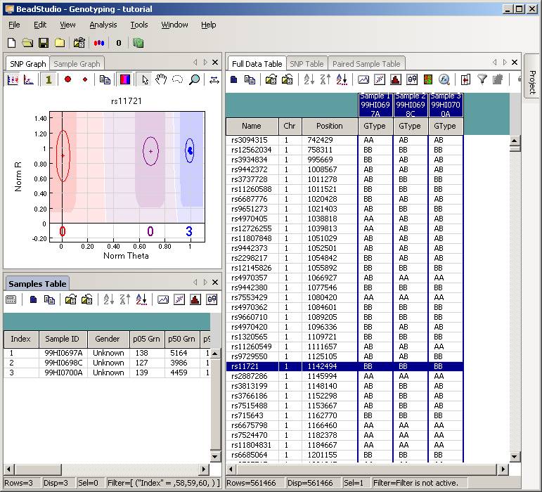
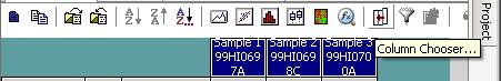
Click the “Column Chooser …” button in the tool bar (the third button to the right), and the column chooser window will appear. Then select the desired columns (GType, Log R Ratio and B Allele Frequency) to be included in output files. For example, if you see that the “B Allele Freq” is shown in the “Hidden Subcolumns” box, you can select it, then click the “<=Show” button, so that it can be moved to the “Displayed Subcolumns” box. The “Displayed Columns” box should contain at least the “Name” field and all individual identifiers. It is strongly recommended to also include “Chr” and “Position” field here. You can hide things like “Address” and “Index” and move them to the “Hidden Columns” box.

Now the BeadStudio window looks like below. Click the “Select All Rows” button (first button in the tool bar) to select all data:

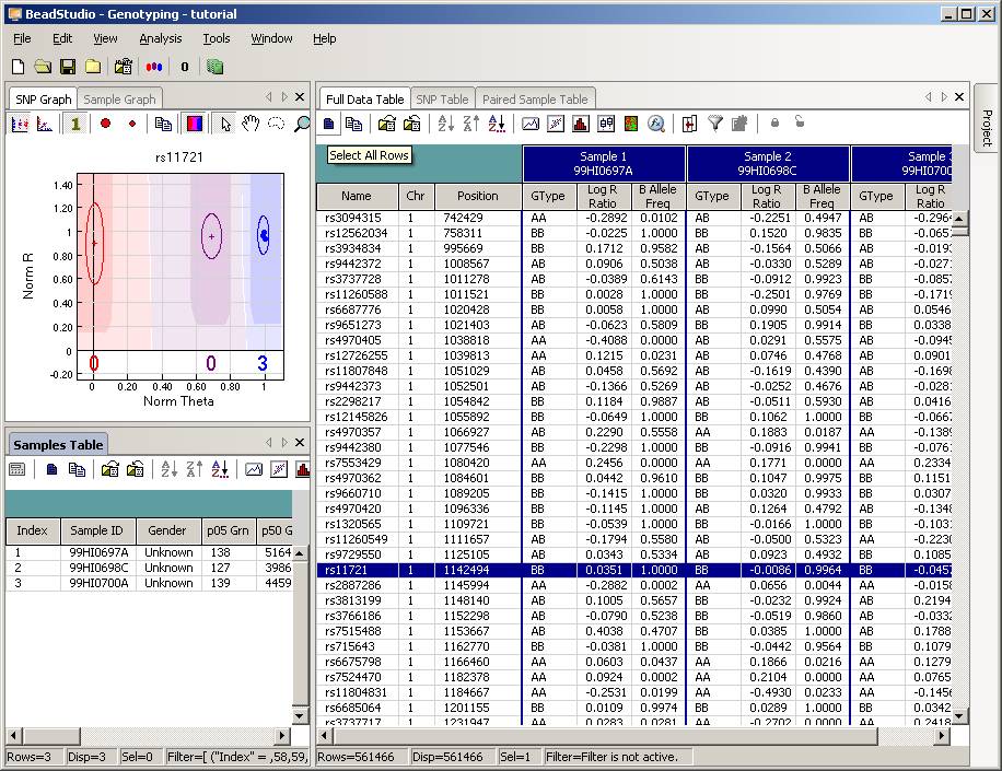
Then click the “Export Displayed Data to File” button (the third button in toolbar), and save the file as something like tutorial.txt. This file will be a tab-delimited file, with one SNP per line, and each line contains genotype, log R Ratio and B Allele Frequency information for all individuals. (If you are using BeadStudio version 3, there will be a dialog asking whether you want to export all data, clicking either “Yes” or “No” is fine, since you have already selected all data). The file size for tutorial.txt is about 50MB for three individuals.

Now transfer the tutorial.txt file to a machine where PennCNV is installed, and we will use the PennCNV software to generate CNV calls for these three individuals.

In the next step, we will process the tutorial.txt file containing genotype data and split the file into individual files. The tutorial.txt file could be exported from BeadStudio software (as done in step 1), or downloaded directly from the PennCNV website Download page (when the user skips step 1).

Next we will process the tutorial.txt file and split it into several files.

The first a few lines of the tab-delimited tutorial.txt file look like this:

The first line is referred to as the “header” line, which contains information on the meaning of each column. Each subsequent line contains information on one SNP per line for all individuals.

We will need to split the file into several files, one for each individual. We can use a standard Linux command “cut” to do that:

The above commands take the desired tab-delimited columns in the tutorial.txt file and generate a new 6-column file for each sample. The first three columns (Name, Chr, Position) in the original tutorial.txt file is kept in all output files.

Alternatively, if the input file is very large (for example, a 6GB file containing genotyping information for 600 individuals), it is very slow to run the “cut” command many times due to the overhead of scanning hard drives (for example, scanning 3.6 terabytes of data). Instead of using the “cut” program, we can use the kcolumn.pl program in the PennCNV package to achieve the same goal but only scan the inputfile file once:

[kai@adenine tutorial1 ENS40]$ kcolumn.pl tutorial.txt split 3 -heading 3 -tab -out sample

The above command specifies that we want to split the tutorial.txt file by tab-delimited column, and the first 3 columns are heading columns (columns that are kept in every output file), and every 3 columns will be written into a different output file. The --tab argument tells the program that the tutorial.txt file is tab-delimited (by default, the kcolumn.pl program use both space and tab character to define columns), and the --out argument specifies that the output file names should start with “sample”. Note that you can use both double dash or single dash in the command line (so --output has the same meaning as -output), and you can omit trailing letters of the argument as long as there is no ambiguity with another argument (so the --output argument has the same meaning as the -o or -ou or -out or -outp or -outpu argument). Also note that if the input file is extremely large (for example, a 12GB file containing genotyping information for 1,200 individuals), we may need to use the --start_split and --end_split arguments and run the kcolumn.pl program multiple times to overcome limitations on simultaneous file handles imposed by the operating system. For example, you can run the program twice: the first time using “-start 1 -end 1000” and the second time using “-start 1001 -end 2000”.

By default the output file names will be appended by “split1”, “split2” and so on; however, you can use the -name_by_header argument (or simply -name argument) so that the output file name is generated based on the name annotation in the first line of the tutorial.txt file.

Tip: The -name argument tells the program that the output file name should be based on the first word in the first line of the inputfile (for example, 99HI0697A and 99HI0698C). Sometimes the sample name contains non-word characters such as "-"; in this case, you can also add the "--beforestring .GType " argument to the above command in addition to the -name argument; this means that any string before the ".GType" should be used as output file name, so that the output file names are sample.99HI0697A, sample.99HI0698C and so on.

To get more detailed description of each argument for the kcolumn.pl program (or any other program in the PennCNV package), try the --help argument. To read the complete manual for the kcolumn.pl program (or any other program in the PennCNV package), use the --man argument.

Now we have three files, called sample1.txt, sample2.txt and sample3.txt, corresponding to three individuals, respectively, and we need to identify CNVs for them.

Note: After file spliting, it is very important to check the output files. Normally, if you keep the terminal open, after the program finished, there should be a line saying that all splitting is done to confirm that this step is completely successfully. Sometimes due to lack of hard drive space, or due to an interruption of the program before it's finished, the file splitting is not completed successfully, resulting in fewer markers than it should contain. You can do a simple "wc -l file.split1" to check the number of lines in a random output file: it should be around 1.8 million for Affy 6, 900K for Affy 5, 1 millino for Illumina 1M and 550K for Illumina 550K array. If not, then the file splitting is not completely corrrectly and you can use "tail file.split1" to see what's the last line in the file, usually the line is not complete, meaning that something is wrong there. Re-do the splitting again, and make sure that the file splitting is completed before calling CNVs.

Preparing signal intensity files from Affymetrix CEL files

The procedure for converting Affymetrix CEL files to the PennCNV input formats are described in detail in the PennCNV-Affy tutorial. This procedure requires the Affymetrix Power Tools (APT) to work.

Preparing signal intensity files from other types of arrays (Agilent, Nimblegen, Affy, etc)

The procedures described above are suitable for standard Illumina and Affymetrix arrays. Sometimes we may encounter different arrays (such as oligonucleotide arrays from Nimblegen and Agilent), or we may have access only to quantitative signal values for each marker, rather than raw CEL files for Affymetrix array (so APT cannot be used). The latter situation is quite common for publicly available data sources, where data providers typically hesitate to give out raw CEL files and instead only gives signal intensity values calculated by their own algorithms.

PennCNV can still process these types of arrays or data using the PennCNV-Affy framework, but the user need to prepare appropriate input file formats. Below is a description of these data formats: in fact they match the same format as output files given by APT, so that PennCNV-Affy can be directly applied on these files.

Normalized signal file

The user need to provide a normalized signal file, possibly by a simple re-formatting of the original file received from data provider. The file has a simple tab-delimited text format: first line gives the sample identifiers, while following lines gives signal intensity values. The first field must be “probeset_id”. In addition, all values must be log2 based, and negative values are possible. It is very important that this file has been normalized (any algorithm should suffice) so that the signal intensity between different samples are comparable to each other: a simple way to check this is to get all intensity values for sample1, calculate its median, 25% and 75% quantile, then compare that of sample2 and sample3 to make sure that they are largely comparable.

If the marker name ends with “-A” and “-B”, it will be treated as a SNP, so two lines will be required to describe its signal intensity values. Otherwise, the marker will be treated as a non-polymorphic marker (CN marker), and only one line is required to describe its signal intensity values. For example, the rs11127467, SNP45265 and marker4438516 above are all SNP markers, while the CN10000 is a CN marker.

Genotype call file

This file is required even if using an oligonucleotide array. It is also a tab-delimited text file, with one marker per line. The first line gives the sample identifiers, while following lines give the genotype calls. The first field again must be “probeset_id”. The order of the samples in this file should match that in the signal file, even if the actual sample name differ.

In the genotyping call field in the file, 0 means AA, 1 means AB and 2 means BB call. CN markers are obviously not included in the file since they have no genotype calls.

Genotype confidence file

This file is required even if using an oligonucleotide array. The format is similar to the above genotype call file. The confidence value are quantitative values, and the smaller, the better (this is somewhat counter-intuitive, but the file format is based on Affymetrix genotyping calls). If using a genotype callingn algorithm (such as Chiamo) that gives higher scores to more confident calls, then the user need to reformat the field to be 1-score, to reflect that lower scores means better call quality.

Generating cluster file and LRR/BAF file

PFB (Population frequency of B allele) file

This file supplies the PFB information for each marker, and gives the chromosome coordinates information to PennCNV. It is a tab-delimited text file with four columns, representing marker name, chromosome, position and PFB values. When PFB value is 2, it means that the marker is a CN marker without polymorphism. An example is given below:

Note that different array manufacturers (such as Affymetrix and Illumina) may use different definition of “B” allele even for the same SNP.

When reading the signal intensity file, PennCNV will only process markers annotated in the PFB file. Therefore, if we want to remove some markers from CNV analysis, due to their low quality, known issues (within segmental duplication region, or within pseudo-autosomal region), we can simply remove these markers from the PFB file, without changing the signal intensity file per se. Similarly, if we want to call CNV on a different genome assembly (NCBI36 versus NCBI35), we can simply change the PFB file to reflect the new chromosome coordinates, without the need to change signal intensity files.

HMM file

The HMM file supplied the HMM model to PennCNV, and tells the program what would be the expected signal intensity values for different copy number state, and what is the expected transition probability for different copy number states. An example is given below:

The first large block (A) specifies the transition probabilities. However, in PennCNV, the transition probability depends on the distance between neighboring markers. Therefore, the numbers here is the average number for a 5kb distance, and the actual transition probability is calculated using previously described formula that adjusts for distance.

The second large block (B) is not used by PennCNV (the very original PennCNV program was adapted from the UMDHMM framework that use this format of HMM model file, so for compatibility with previous versions, the same HMM format is used in all updated version, despite that fact that many fields are just useless). The pi values specify the initial probability for different copy number states in the HMM chain.

The third large block (B1, B2, B3) specifies the expected (mean) signal intensity values, as well as their standard deviation. B1 is used for LRR, B2 is used for BAF, while B3 is used for LRR of CN markers which typically have larger variance than SNP markers. The two signal intensity values, including LRR and BAF, are both used by PennCNV. Furthermore, a UF factor is used by PennCNV that specified the fraction of expected “bad” markers, that is, markers that behave badly and do not meet expectation. For Illumina arrays, 0.01 seem to be a good choice; for Affymetrix arrays, this value should be slightly higher to 0.03 or 0.05. Obviously, this value reflects the “sensitivity” of the calling algorithm especially on very small CNV regions: when higher UF value is used, the signal from smaller yet real CNV region may be treated as random noise in the data but the algorithm is more robust to random fluctuation of signal values).

GCModel file

This file specifies the GC content of the 1Mb genomic region surrounding each marker (500kb each side). It is used by the -gcmodel argument in PennCNV, and has been useful to salvage samples affected by “genomic waves” (see Diskin et al for details). An example is given below:

Note that the second and third column are not used by PennCNV, since the information is already provided in the PFB file. The GC values range from 0 to 100, indicating the percentage of G or C base pairs in each region surrounding the marker.

List file

Although the signal file names can be supplied in command line, the -list argument in PennCNV can take a list file that gives all file names to be processed.

When calling CNV for each individual, the list file should contain one file name per line. When calling CNV for trios (using -trio argument or -joint argument), the list file should contain three file names per line separated by tab character. When calling CNV for quartets, the list file contains four file names per line separated by tab character.

If the file name in list file is enclosed by the ` character, it will be treated as a system command instead, rather than a file name. PennCNV will execute this system command, read the signal values from this command, and then generate CNV calls. One obvious example is to store signal values in a compressed file (for example, sample1.txt.gz), and then use `gunzip -c sampl1.txt.gz` as the input file name to PennCNV. Alternatively, some centers may store all signal intensity values in a relational database, and write custom scripts to retrieve these signal values and output in tab-delimited format. In such cases, these custom scripts can be specified in the list file in the above manner for PennCNV to process directly.